Shapefile drawing using Python
Last week, I needed to draw some maps and display data on these maps also. I have spent some hours to discover how to complete this task. Thus, in this post, I will summarize step by step to accomplish the initial goal.
Basic drawing
- First time first, we need to download the shapefile before doing anything. Luckily, Open street map is an open source data for us to download the shapefile of boundary of many countries. However, there are some services extracted the shapefile of each countries for us. The data is quite complete and ready to use. I also put the demo data of Singapore link1 link2 link3, and they are used to illustrate latter steps (please download the whole three).
- Secondly, we need to choose the library to draw. BaseMap is a common lib for drawing shapefile but it is overkilled in my situation i.e. I do not need to use its fancy features. Thus, pyshp is my selection. It is lightweight but still powerful enough to satisfy my requirement. Moreover, installation and usage are as easy as ABC :-) . Last but not least, I have used Python 2.7 and matplotlib 1.4.2 to draw but the conversion to Python 3.x is not hard.
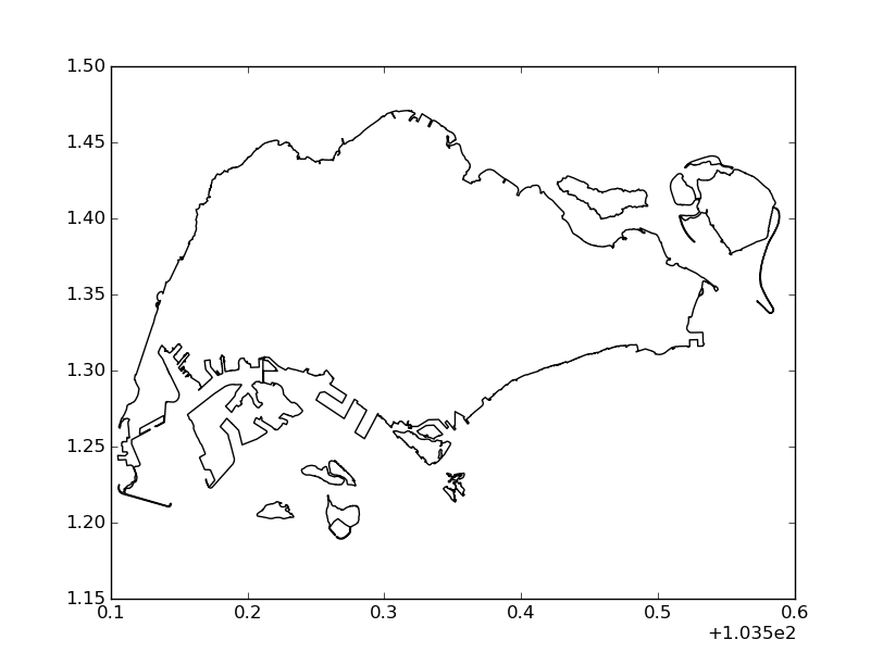
- Let us draw :-D
# import libraries
import shapefile as shp
import matplotlib.pyplot as plt

#load shapefile
sf = shp.Reader('SGP_adm0.shp')

plt.figure()
for shape in sf.shapeRecords():

    # end index of each components of map
    l = shape.shape.parts

    len_l = len(l)  # how many parts of countries i.e. land and islands
    x = [i[0] for i in shape.shape.points[:]] # list of latitude
    y = [i[1] for i in shape.shape.points[:]] # list of longitude
    l.append(len(x)) # ensure the closure of the last component
    for k in xrange(len_l):
        # draw each component of map.
        # l[k] to l[k + 1] is the range of points that make this component
        plt.plot(x[l[k]:l[k + 1]],y[l[k]:l[k + 1]], 'k-')

# display
plt.show()
The final result is not bad.
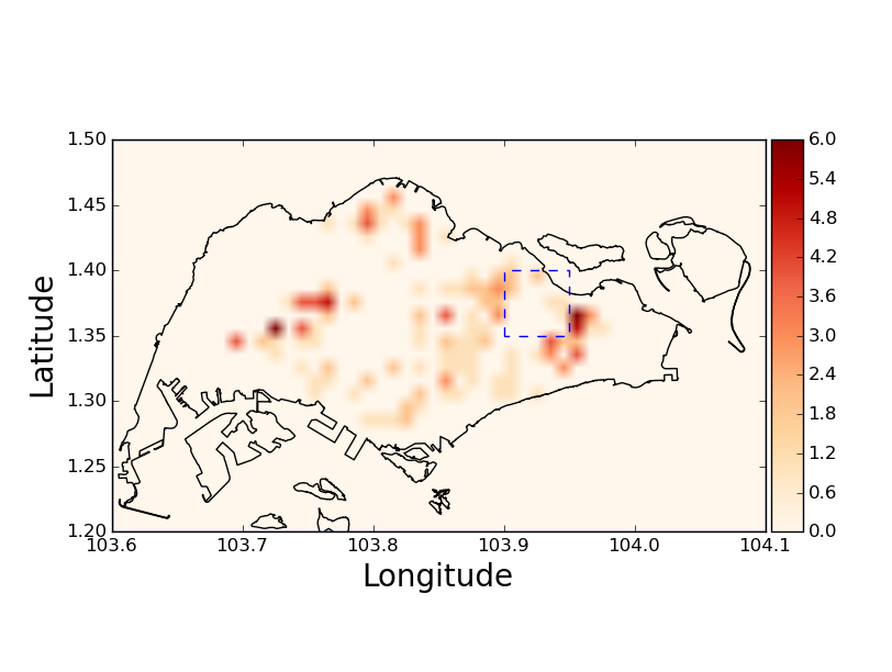
Display histogram
Using the same setup as above, we will display the histogram in 2D map to illustrate the density. There are some tricks to complete the task so let us view the code first.
import shapefile as shp
import matplotlib.pyplot as plt
import matplotlib as mpl
from mpl_toolkits.axes_grid1 import make_axes_locatable
import numpy as np

def drange(start, stop, step):
    result = list()
    r = start
    i = 0.0
    while r < stop:
        result.append(r)
        i += 1.0
        r = round(start + i * step, 3)
    result.append(r)
    return result

def readLoc(fname):
    f = open(fname, 'r')
    lines = f.readlines()
    f.close()
    x = list()
    y = list()
    for line in lines:
        comp = line.strip('\n').split(',')
        x.append(float(comp[1]))
        y.append(float(comp[0]))
    return x, y

#load shapefile
sf = shp.Reader('SGP_adm0.shp')

plt.figure()
for shape in sf.shapeRecords():
    l = shape.shape.parts
    len_l = len(l)  # how many parts of countries i.e. land and
    x = [i[0] for i in shape.shape.points[:]]
    y = [i[1] for i in shape.shape.points[:]]
    l.append(len(x))
    for k in xrange(len_l):
        plt.plot(x[l[k]:l[k + 1]],y[l[k]:l[k + 1]], 'k-')

lower_x = 103.6
lower_y = 1.2
upper_x = 104.1
upper_y = 1.5
# plot the frame of city
x = [lower_x, lower_x, upper_x, upper_x, lower_x]
y = [lower_y, upper_y, upper_y, lower_y, lower_y]
plt.plot(x, y)

# load data
fname = '1.35_103.9_1.4_103.95'
comp = fname.split('_')
loc = [float(i) for i in comp]
x, y = readLoc('user_density.txt')

# plot the line
area_x = [loc[1], loc[1], loc[3], loc[3], loc[1]]
area_y = [loc[0], loc[2], loc[2], loc[0], loc[0]]
# plot a box in map
plt.plot(area_x, area_y, 'b--')

# histogram
xedges = drange(lower_x, upper_x, 0.01) # 0.01 is the size of bin
yedges = drange(lower_y, upper_y, 0.01)
H, xedges, yedges = np.histogram2d(x, y, bins=(xedges, yedges))

im = plt.imshow(H.T, cmap='OrRd', interpolation='bilinear', origin='low', extent=[xedges[0], xedges[-1], yedges[0], yedges[-1]])

# add label to axis and do not scale unit of x, y axises
plt.ylabel('Latitude', fontsize=20)
plt.xlabel('Longitude', fontsize=20)
ax = plt.gca()
ax.ticklabel_format(useOffset=False)
divider = make_axes_locatable(ax)                          # set size of color bar
cax = divider.append_axes("right", size="5%", pad=0.05)    # set size of color bar
plt.colorbar(im, cax=cax)                                  # set size of color bar

# finally, show the plot
plt.show()
The file user_density.txt could be downloaded via this link. The data inside this file is generated randomly. Each line of file contains 2 information latitude and longitude of each point and both are separated via comma. Function readLoc is used to load its data.
There are 2 important notes for the above code
- I do not use the normal order in numpy manual which is (y, x)
H, xedges, yedges = np.histogram2d(x, y, bins=(xedges, yedges))
- We use the transpose matrix of
H.Twhen usingimshow. Optionbilinearis used to make it look like heatmap.
im = plt.imshow(H.T, cmap='OrRd', interpolation='bilinear', origin='low', extent=[xedges[0], xedges[-1], yedges[0], yedges[-1]])
The final result is quite beautiful